
Excel Spreadsheets: Tables
Introduction
We all know that Excel uses Rows & Columns as its structure, and some would also think that by adding Borders and Headers to our data, we have created a table. And as much as it may ‘look’ like a table to us……..Excel does not recognise it as a Table.
However, when we do use Tables (as Excel sees them), we actually unleash more power over our data, so there are plenty of advantages to using them. Some would even argue that using Tables is the ONLY way to use Excel.
Let’s explore them in a little more detail and you can decide for yourself.
What Are Tables in Excel?
Tables represent a ‘structured range of data’ that Excel recognises as ONE single entity.
They have powerful features such as: Excel immediately applies filters, formatting, and treats your data as a dynamic entity that adjusts and expands as needed.
A Table is NOT just formatting — it’s a special Excel object that brings structure, intelligence, and automation to your data.
Is this a table?
Screenshot1
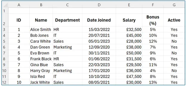
This is NOT a Table, this is merely just the use of cells.
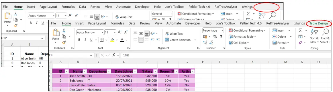
There are a few ways to identify a Table, but the first, most obvious signal, is the absence of the ‘Table Design’ ribbon at the top of the screen.
If this WAS a table, the ‘Table Design’ ribbon would ALWAYS be visible once any cell within the Table is selected.
Screenshot2
How to create a Table?
Tables are super simple to create:
- Select all of your data (including header row)
- Go to ‘Home’ ribbon
- Select ‘Format as Table’
** Alternatively to the above, select any cell within the range and press Ctrl + T **
- Select required format (this can be changed later)
- Confirm Range, and that the Table contains headers (on first row)
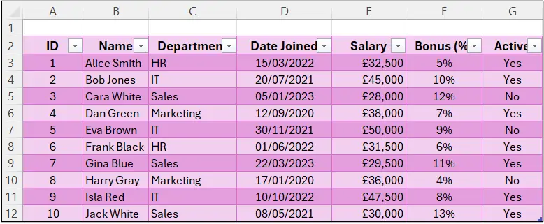
The data will be converted to a Table and will appear similar to this:
Screenshot3
Why Use Tables?
The most obvious change is that each row is now sequentially coloured, making the data easier to read, but there are some other changes that have taken place too:
- Automatically applied Filters (and will also expand if rows and columns extend)
- Automatically applied a ‘Named Range’ i.e. Table1 (and will also expand if rows and columns extend)
- As a new column is added, the Table will automatically include headings
- As a new row is used, the formatting, formulas and data validation will be copied and applied
- As a formula is entered (or amended), it will automatically be applied to all rows, using Structured Referencing, instead of absolute cell references.
- Automatically freezes Headers, so as you scroll down, the column letters will be replaced with the Headers
Working with Structured References
If we want to include a new column to calculate the Bonus Value, we can start by entering the column header into cell H2. Once we do this, the Table will automatically expand to include column H, as shown below:
Screenshot4
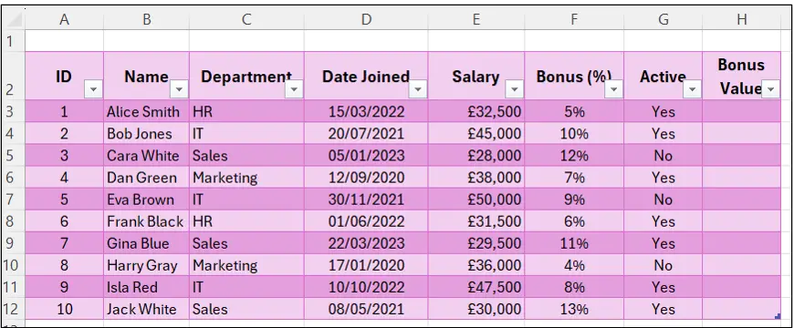
The formatting, filters and named ranges are all extended to column H automatically, simply as a result of adding the new header.
In cell H3, we want the formula =E3*F3, but as we type it and select the relevant cells, the formula becomes: =[@Salary]*[@[Bonus (%)]].
This is because it is using ‘Structured References’ which reference column headers instead of specific cells. Structured Referencing automatically applies the formula to the correct row within the Table.
Notice as well that as soon as we press ‘Enter’, the formula is automatically copied into EVERY row of the Table.
Benefits of Structured Referencing
- More readable and meaningful formulas
- Automatically updates as data changes, and applies to entire column
- No need to manually copy formulas (or risk forgetting)
- No need to include fixed cell references (with dollar symbols)
- Structured References automatically adjust formulas outside the table too, so VLOOKUPs, SUMIFS, etc., stay correct even as the table grows.
Tips and Best Practices
Always use relevant names for Tables (Formulas ribbon >> Name Manager or Table Design >> Table Name).
Avoid merged cells in tables, instead use formatting tricks like Center Across Selection.
Use slicers for fast filtering (it is not possible to use slicers without a Table (or Pivot Table)).
Limitations
- Tables cannot be created within Tables (i.e. nested). It is possible to have lots of separate tables, but not one table inside another.
- The Subtotal function cannot be used within Tables
- Formatting may behave oddly if pasted over or heavily altered.
- New data will always be added to the Table, which makes it difficult to make a one-off calculation within the sheet. (If you leave a blank row or column between the Table, this data won’t be added to the Table.
Common Mistakes
- Structured references can confuse beginners at first. They may not realise that formulas behave differently.
- Using Merged Cells within a Table
- Forgetting to name (or rename) Tables properly, can make complex formulas more difficult to manage later.
Conclusion
Tables reduce errors and save time by automatically expanding to include new data, keeping formulas, formatting and references consistent.
They increase flexibility by allowing easy sorting, filtering, and dynamic referencing without needing to constantly adjust ranges.
Tables support automation by working seamlessly with Power Query, PivotTables, and dynamic arrays, making data updates fast, accurate, and hands-free.
In short: Tables turn simple data into living, breathing Excel tools — and learning to master them is a major upgrade for any spreadsheet user.
This article was written by Traci Williams and originally published by Executive Support Magazine.