
You’ve probably heard of data validation in Excel before. This is the process of setting rules or criteria to restrict and ensure the accuracy and integrity of data entered into cells.
This is useful because it helps to prevent errors, ensures consistency, and enhances data accuracy by allowing you to define and enforce specific criteria for the input of information.
Dependent data validation in Excel takes this one step further and gives us the ability to create a dynamic relationship between two or more cells, where the options available in one cell depend on the value selected in another cell.
This feature is particularly useful when you want to streamline your data entry and ensure accuracy by limiting choices based on specific criteria.
For example, if you have a worksheet with countries and corresponding cities, you can set up dependent data validation to display only the cities relevant to the selected country (and I’ll walk you through this shortly).
By establishing these dependencies, you can make accurate and consistent selections, which reduces the risk of errors in your data entry and enhances the efficiency of your data management.
Picklists are a commonly used form of data validation in sheets. They create a dropdown list that we can choose from to help us streamline our data entry process. They’re extremely useful and can be a massive time saver (which is always a plus in my book).
Dependent data validation goes one step further than just creating a series of picklists that we have to manually select from. If you have multiple picklists with data that is linked (think back to the countries and cities) you can use dependent data validation to help narrow down your choices when it comes to your secondary list.
For example, if our first picklist has a list of countries, we can use this formatting to then make the second list only show cities that are from the selected country.
I’m going to walk you through this example in more detail. You can either follow along with my written instructions or watch the following video for guidance:
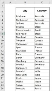
Before you can create your dependent data validation, you’ll need to organise your data. For this example, I’ve created a table that lists countries in one column and cities in the next.
I’ve organised my table by country (from A-Z), and have offset the cities column to match the countries they sit alongside.
To get started with our dependent data validation we’re going to create a ‘named range’ for the countries.
To do this, highlight all the cells in the ‘Country’ column, including the heading, then go to the Formulas tab in the ribbon, find ‘Create from Selection’, make sure ‘Using the top row’ is selected, and then click ‘OK’.
You’ve now created a named range called: Country. If you go into ‘Name Manager’ in the Formulas ribbon, you’ll now be able to see (and amend) this named range.
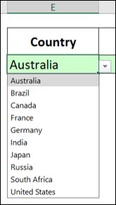
Next, go to the empty cell where you want to add your data validation. Click into the cell, then go to the Data ribbon, and select ‘Data Validation’.
In the Data Validation window, select ‘List’ from the drop-down menu under ‘Allow’. Next, in the box under ‘Source’ you can now press F3 and choose from a list of your named ranges (which is where you’ll want to select Country).
By choosing these options, you’re restricting the data that can appear in your selected cell to only come from the Country column of your table.
You’ll now have a picklist in your selected cell that shows you all of the data from the Country column.
Now that we can choose a Country from our picklist, we want to create a secondary picklist that will display the Cities that are matched with that country in our table.
To do this, I’m going to use the following formula:
=OFFSET($B$3,MATCH($E$3,$C$3:$C$32,0)-1,0,COUNTIF($C$3:$C$32,$E$3),1)
Now, I know this looks scary, and a lot of people hate this, but trust me, using dependent data validation isn’t as difficult as this formula might look at first glance.
The formula above uses the specific cell ranges and information for the example I’m working through, but I’ll break it down for you below to help you create your own.
The syntax of this formula is OFFSET(reference, rows, columns, [height], [width]). To break this down even further, here’s what each part of this formula means:
When we put this together in the example above, what we’ve instructed Excel to do is to:
Once you’ve inputted this formula, you will see that a new list is created that shows the matching Cities for your selected Country.
To turn this into a picklist, go into the Data ribbon and select ‘Data Validation’.
In the ‘Data Validation’ window, select ‘Allow’ > ‘List’ and then in your ‘Source’ box, paste the formula you’ve just created and click ‘OK’.
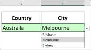
You’ll now see that you’ve created a picklist that displays the matching Cities to the country chosen from your first picklist. (If you haven’t selected a country, you won’t see anything in your city picklist, because it’s dependent on having a matching column).
HINT: I always recommend writing the formula out in a blank cell before adding it to your data validation so that you can test it to generate the correct list – this helps me wrap my head around it and makes sure that my data validation will be able to work correctly.
The great thing about using this formula as a picklist is its ability to dynamically calculate the data it displays. If you were to add new cities to your table, this formula will recognise the additions and will automatically update your picklist – isn’t that ACE?
To help you get to grips with dependent data validation and use this formula to create your own picklists, you can download the completed sheet I’ve used as an example in this article. Click here to download.

