
Excel Spreadsheets: Sort & Filter Formulas
Introduction
Using Excel’s functions ‘Sort’ & ‘Filter’ are fairly second nature to us now, they tend to be used daily by most people who use Spreadsheets.
But, did you know that we can now use these features as FORMULAS to extract data from the source? They’re pretty ACE!!
They are perfect if you want your raw data to remain untouched, but build external summaries from it.
SORT Formula
This formula will dynamically extract a list of values sorted in a specified order (Ascending, Descending etc) using a Formula, and NOT the Function, from the raw data. The DYNAMIC nature of this formula, means it will continually update (and expand or contract) as the raw data changes, without any manual intervention.
In this example, we have a simple list of Names of Sales People:
Screenshot1
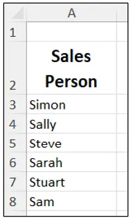
We can use the ‘Sort’ formula to extract this list, and sort it into alphabetical order, as follows:
- Select a cell where you want the list to start form (e.g.C3)
- From ‘Formulas’ ribbon (1), select ‘Inset Function’ (2), then type ‘Sort’ (3) and click ‘Go’ (4) :
Screenshot2
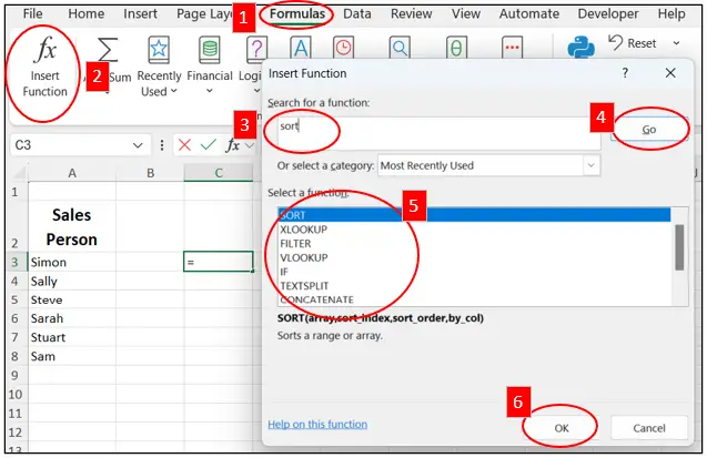
A list of ‘potential’ formulas will appear at the bottom, select the one called ‘Sort’ (5), then click ‘OK’ (6).
The wizard will appear to guide you as to what to enter:
Screenshot3
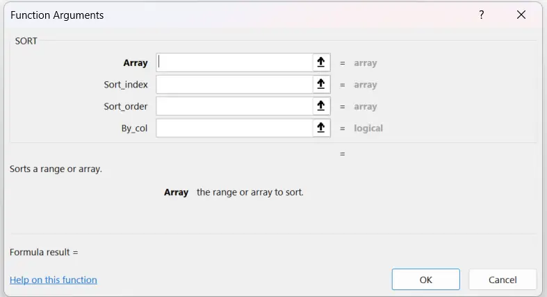
The boxes should be completed as follows:
Array
Enter the ‘Range’ to be used i.e. A3:A8
The next 3 boxes are optional as follows:
Sort_Index
This is a number indicating the row or column to Sort By (this is usually obvious from the selected range)
Sort_Order
This is the basis of Sort (1 = Ascending (default), -1 = Descending)
By_Col
This is the SORT Direction (FALSE = by Row (default), TRUE = by Column)
Then click OK and the formula (and result) would appear like this:
Screenshot4
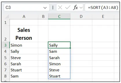
The formula ONLY includes the Array (=SORT(A3:A8)) as none of the other optional fields were relevant in this instance, and the list now appears in alphabetical order (ascending).
Of course, if I wanted the list to appear in descending order, I could simply amend the formula like this:
Screenshot5
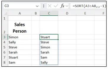
This formula only appears in the first cell (C3), and is ‘SPILLED’ into the rows below using as many rows as there is data. This is the DYNAMIC nature of this formula.
The benefit of this, is that if the list of Names in column A expands or reduces (inserting or deleting rows), so too will the SPILLED range in column C…..without the need for any manual intervention.
This also means that this formula does not need to be copied down into multiple rows, and Excel is not having to perform multiple calculations, making the processing quicker, and keeping the file size low.
SORTBY Formula
With this formula it’s possible to define the criteria to sort by (not just base it on the source range).
In this instance, we might want to SORT the Sales Person into the order with the highest Sales:
Screenshot6
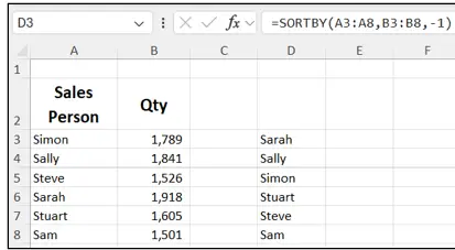
The syntax of this formula would be:
Screenshot6a

Array
Enter the ‘Range’ to be used i.e. A3:A8
By_Array1
This is the range by which to sort the data i.e. B3:B8 (Qty)
The next box is optional as it will default to ‘Ascending Order if non populated:
Sort_Order1
This is the desired sort order 1= Ascending Order / -1 = Descending Order
The result would appear like this:
Screenshot7

You can also add multiple criteria if required too.
FILTER Formula
Just like SORT, the FILTER formula also works dynamically and will extract data based on defined filter criteria.
In this example, we have lots of data and we might want to extract all of the data for Customer D:
Screenshot8
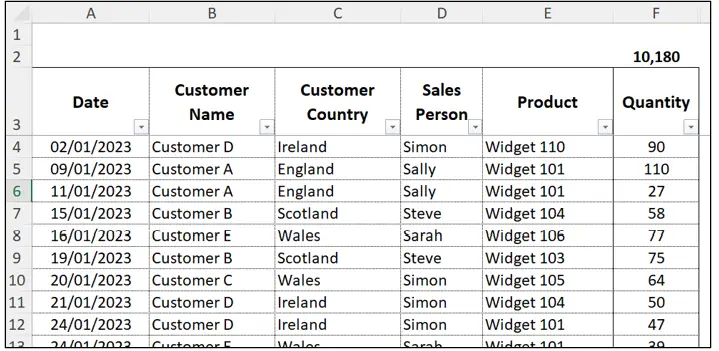
Of course, we could apply a Filter directly on the raw data, but this would temporarily hide all other rows, preventing us from seeing those.
This is where we can use the ‘Filter’ formula to extract the data for that Customer:
- Select a cell where you want the data to start form (e.g.H3)
- From ‘Formulas’ ribbon, select ‘Inset Function’, then type ‘Filter’ and click ‘Go’
- A list of ‘potential’ formulas will appear at the bottom, select the one called ‘Filter’, then click ‘OK’:
The wizard will appear to guide you as to what to enter:
Screenshot9
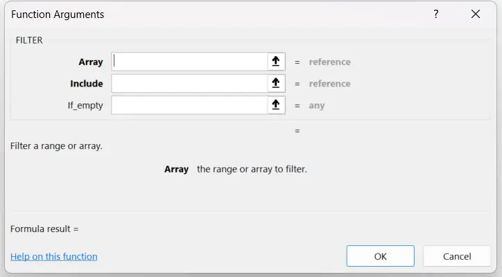
The boxes should be completed as follows:
Array
Enter the ‘Range’ to be used i.e. A3:F201
Include
Enter the criteria to be filtered by i.e. B3:B201=”Customer D”
The next box is optional:
If_empty
This is the opportunity to tell the formula what to return if it is unable to find a match for the criteria. This will return an error if not defined.
- Click OK
The result would appear like this:
Screenshot10
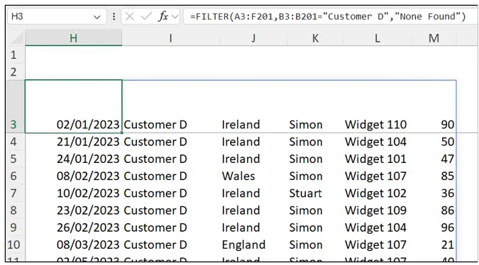
Notice that I have used the Array: A3:F201, meaning that this will return ALL of the columns. I could have made the Array: A3:C201 and this would have just returned the 1st 3 columns.
The ‘None Found’ part of the formula is what would be returned if there was no data matching that criteria.
As with the ‘Sort’ formula, you can see that the formula is only entered into the 1st cell (H3) and then SPILLS into the remaining cells as appropriate, returning all the columns of data, ONLY for those rows that include ‘Customer D’.
We can literally amend the Customer Name in that formula to easily and quickly return a different subset of data.
Of course, if any of the raw data was to update, then the result of the FILTER formula would also automatically update too.
We may prefer to filter the list based on a Product instead, and to do this, we would simply amend the contents of the ‘Include’ part of the formula, as follows:
Screenshot11

It may also be a requirement to filter by BOTH Customer AND Product, and this would require a slight modification to the ‘Include’ part of the formula, as follows:
Screenshot12
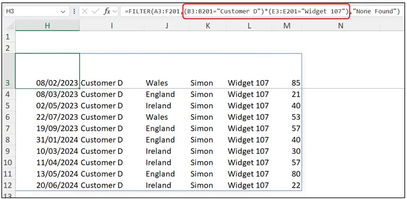
Notice the part of the formula highlighted with the red box contains BOTH the Criteria for filtering by Customer & Product, both in brackets, and joined with an asterisk ( * ). This means that BOTH conditions must be met.
You can include multiple criteria in this formula.
Top Tip:
Using * applies AND logic (i.e. ALL conditions must be met).
Using + applies OR logic (At least one condition must be met).
Multiple conditions can be included inside the include argument.
Conclusion
These formulas provide powerful ways to organise and analyse data dynamically, as unlike manual sorting and filtering, these functions automatically update when the source data changes, saving time and improving efficiency.
With practice, dynamic sorting and filtering can transform how you work with data in Excel, making complex tasks simpler and more efficient.
This article was written by Traci Williams and originally published by Executive Support Magazine.