
Excel Spreadsheets: Dynamic Arrays
How one formula can do the work of dozens — and make you look like an Excel ACE.
We are used to writing formulas, pressing enter, and then copying them down rows or across columns. But in the latest versions of Excel (Microsoft 365), there’s a new way to manage this: Dynamic Arrays.
With these, you write one single formula in one cell, press Enter… and Excel instantly spills the results into multiple cells. No dragging. No copying. Just instant results.
AND, it will automatically expand or reduce the range as and when the data changes too.
Dynamic Arrays are one of the biggest Excel upgrades in 30 years — but many users don’t even know they exist.
Dynamic Array Functions
Here are the 5 most powerful ones to start with — and how they can transform everyday tasks:
- UNIQUE()
What it does: Removes duplicates from a list
EA Use Case: Create a clean attendee list from a messy sign-up sheet
- SORT()
What it does: Automatically sorts data as it changes
EA Use Case: Keep Names sorted in alphabetical order
- FILTER()
What it does: Returns only rows that meet specified criteria
EA Use Case: Pull out all bookings for a specific Event / Location
- SEQUENCE()
What it does: Creates number / date sequences instantly
EA Use Case: Generate seating numbers, day lists for conferences, dates for follow up
- (Combinations)
What it does: Combine functions for magic
EA Use Case: SORT(UNIQUE(FILTER(…))) to build dynamic reports
Real-World Example 1: Cleaning an Attendee List
With this list of Names, those highlighted in Pink appear more than once, and there are issues with the capitalisation:
Screenshot1
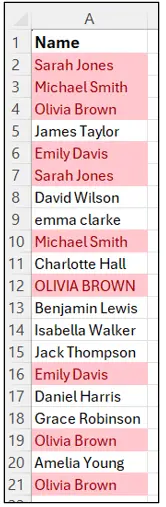
Before:
You copy names into a new column, remove duplicates manually, tidy up capitalisation, then sort them.
After:
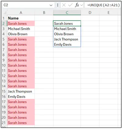
=UNIQUE(A2:A21)
Instantly creates a deduplicated list that updates automatically when new names are added:
Screenshot2

In cell C2 you can see the single formula, and the list of unique values it returns.
The real beauty of this formula is that it automatically spills to row 15, as that is how many Unique Values there are. However, if we were to change the data, the UNIQUE formula would automatically adjust to number of rows it spills into, like this:
Screenshot3
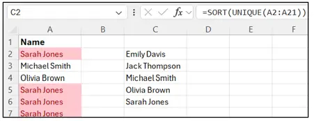
We could also take this formula a step further and make the list SORTED into alphabetical order. The existing formula would literally be wrapped with SORT: =SORT(UNIQUE(A2:A21))
Screenshot4
Real-World Example 2: Instant Reports with FILTER
The data below represents all company bookings, and you are asked:
“Can you give me just the bookings for London?”
Screenshot5
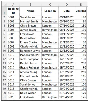
Before: We could apply a Filter to the data and filter column C to only show London
After: We can literally apply just ONE formula to achieve this:
=FILTER(A1:E21,C1:C21=”London”)
Screenshot6
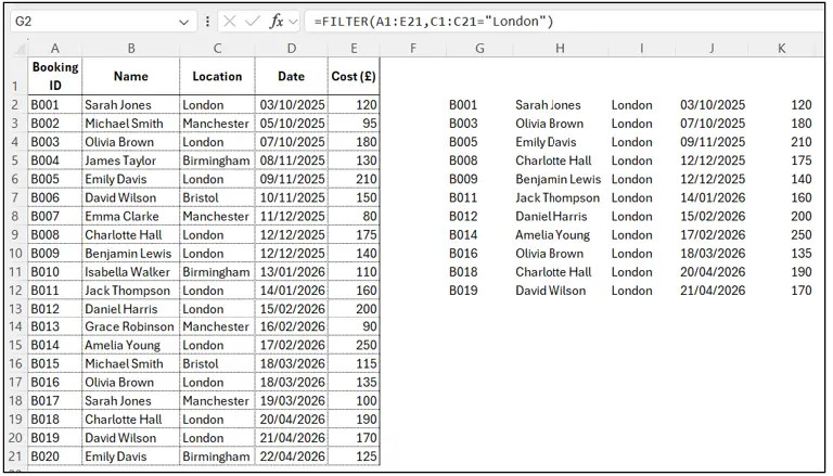
This formula instantly pulls only the matching rows into a neat table. No filters, no copying. This also leaves our original data untouched too.
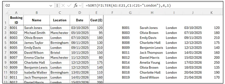
We could SORT the list too?
=SORT(FILTER(A1:E21,C1:C21=”London”),4,1)
This sorts by the 4th column (i.e. Date) in ascending order (1).
Screenshot7
Real-World Example 3: Auto-Numbering and Scheduling
Need a quick numbered list for event seating?
=SEQUENCE(100)
A list of 1 to 100 instantly…….no need for dragging, or Fill Series.
Want dates from 1–31 January 2026?
=SEQUENCE(31,1,DATE(2026,1,1),1)
Or dates for Q1 2026, every other week?
=SEQUENCE(7,1,DATE(2026,1,1),14)
7 represents 7 rows of data (i.e. 7 time periods in a qtr)
14 represents the 14 day intervals
DATE(2026,1,1) represents the start date (amend this if you wanted a specific day)
Real-World Example 3: Combining Functions = Real Magic
Dynamic Arrays have a combined power when you stack the functions together.
For example, to get a sorted list of all unique London attendees:
=SORT(UNIQUE(FILTER(A1:C21, B1:B21=”London”)))
Screenshot8
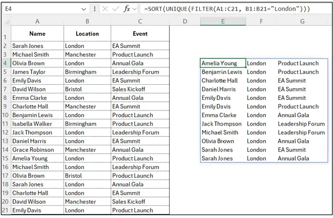
This single formula:
- Filters for London
- Removes duplicates
- Sorts alphabetically
- Updates automatically as data changes
No helper columns. No manual steps. No Filters. One cell.
We can also take this a step further by Filtering for a specific Event as well as Location:
Screenshot9

Here, Users can select the Location AND Event from the pick lists in the green cells, and the relevant data will automatically appear in the table below.
The formula has been updated to:
=SORT(UNIQUE(FILTER(A1:C21, (B1:B21=F1)*(C1:C21=F2))))
B1:B21 = F1 This will filter items in column B that equal the selection in cell F1 (Location)
C1:C21 = F2 This will filter items in column c that equal the selection in cell F2 (Event)
Why Executive Assistants Will Love This
- Huge time saver — less manual copying and filtering of data and formulas.
- Reduces Errors — no forgetting to ‘fill down’ a formula.
- Impressive — looks advanced, but it is simple to use once you know how.
- Reusable — build once, reuse for multiple reports / events.
You’ll look like you’ve built a complex report… when it’s literally just one formula.
Quick Tips
- Dynamic Arrays work in Microsoft 365 and Excel Online (not older versions).
- Where possible, make sure your source data is in a Table — it makes formulas easier.
i.e. =UNIQUE(Names[Name]) instead of =UNIQUE(A2:A21)
- If results ‘spill’ into existing data in your sheet, Excel will show a #SPILL! Error. This means there is not enough space for Excel to ‘SPILL’ the results, so it won’t show any data at all. Clear the data in it’s way and the formula will work as normal.
- Start simple (e.g. UNIQUE()), then layer functions as you grow confident.
Conclusion — Start with One Wow
You don’t have to learn everything at once. Pick one task you do every week, and see if a Dynamic Array can automate it. Once you see that first “wow”, you’ll never go back to copy-pasting again.
Try This Today:
If column A has a list of names, in a blank cell, type:
=UNIQUE(A:A)
Congratulations on your first Dynamic Array!!
If you liked this Article, you won’t want to miss the next one, where we explore even more Dynamic Arrays such as: HSTACK, VSTACK, TAKE, DROP, CHOOSECOLS & CHOOSEROWS.
This article was written by Traci Williams and originally published by Executive Support Magazine.